Análisis de multas de circulación impuestas en Madrid durante Julio 2017
Vamos a analizar el fichero de multas del Ayuntamiento de Madrid, con información sacada del portal de OPenData : http://datos.madrid.es
Como siempre importamos las librerias necesarias : pandas, numpy y matplotlib
import pandas as pd
import numpy as np
import matplotlib
import matplotlib.pyplot as plt
import datetime
import matplotlib.dates as mdates
%matplotlib inline
import matplotlib.ticker as mtick
from matplotlib.ticker import FuncFormatter
pd.options.display.float_format = '{:,.1f}'.format
Preparamos una texto para incluirlo en cada gráfico como fuente…
fuente='Fuente : Ayuntamiento de Madrid, http://datos.madrid.es'
Preparando la URL de la fuente de datos
path_web='http://datos.madrid.es/egob/catalogo/210104-162-multas-circulacion-detalle.csv'
cabecera de las columnas
nombre_columnas=['CALIFICACION','LUGAR','MES','ANIO','HORA','IMP_BOL','DESCUENTO','PUNTOS','DENUNCIANTE','HECHO_BOL','VEL_LIMITE','VEL_CIRCULA','COORDENADA_X','COORDENADA_Y']
Leemos los datos desde su localizacion en ‘path_web’, en este fichero tenemos los datos de Junio de 2017. Al respecto de la la identificacion de la multa en el tiempo tendremos la hora pero no el día del mes, es decir : tendremos las multas puestas a las 13:10 a lo largo de todo el mes, pero no podremos partirlas por día. No encuentro otra razón que no sea evitar cualquier vía de identificación del conductor.
multas=pd.read_csv(path_web,sep=";",encoding='windows-1250',index_col=False,header=None,names=nombre_columnas,skiprows=1)
confirmamos que ha bajado correctamente
multas.columns
Index([‘CALIFICACION’, ‘LUGAR’, ‘MES’, ‘ANIO’, ‘HORA’, ‘IMP_BOL’, ‘DESCUENTO’,
‘PUNTOS’, ‘DENUNCIANTE’, ‘HECHO_BOL’, ‘VEL_LIMITE’, ‘VEL_CIRCULA’,
‘COORDENADA_X’, ‘COORDENADA_Y’],
dtype=’object’)
Convertimos la columna ‘HORA’ con horas tal que 21.30 en datetime
multas['HORA']=pd.to_datetime(multas['HORA'],format='%H.%M')
Añadimos una columna hora_entera, tal que la hora (desde 00 hasta 23) para facilidad de cálculo de algunos gráficos..
for n in range(0,multas.shape[0]):
multas.set_value(n,'hora_entera',multas.loc[n,'HORA'].strftime('%H')+':00');
Hay que tratar un poco los dos campos relacionados con velocidad (limite y velocidad multada:
a) tanto los vaklores de aquellas multas no relacionadas con velocidad en las que el valor es un string de 4 caracteres BS : ‘ ‘
b) Aquellos relacionados con velocidad en los que hay que convertir el string con la velocidad a un integer.
He generado un par de columnas adicionales para contener estos datos ya tratados..
velocidad=lambda x : 0 if x==' ' else int(x.strip())
multas['velocidad_limite']=multas['VEL_LIMITE'].apply(velocidad)
multas['velocidad_circulacion']=multas['VEL_CIRCULA'].apply(velocidad)
multas.columns
Index([‘CALIFICACION’, ‘LUGAR’, ‘MES’, ‘ANIO’, ‘HORA’, ‘IMP_BOL’, ‘DESCUENTO’,
‘PUNTOS’, ‘DENUNCIANTE’, ‘HECHO_BOL’, ‘VEL_LIMITE’, ‘VEL_CIRCULA’,
‘COORDENADA_X’, ‘COORDENADA_Y’, ‘hora_entera’, ‘velocidad_limite’,
‘velocidad_circulacion’],
dtype=’object’)
Empezamos a sacar algunos resultados :
Número total de multas : 235.099 multas en Julio 2017
len(multas)
235099
Cuántos puntos se han perdido en esas multas? : 27.037
puntos_totales=multas.PUNTOS.sum()
print ('Puntos total perdidos: {:,.0f} puntos'.format(puntos_totales))
Puntos total perdidos: 27,037 puntos
Cual es la suma del los importes de esas multas, antes de descuento?
euros_totales=multas.IMP_BOL.sum()
print ('Importe total de multas antes de descuento: {:,.0f} euros'.format(euros_totales))
Importe total de multas antes de descuento: 23,113,010 euros
Cual es el importe de la multa de más y menos importe?
print ('Importe más alto: {:,.0f} euros'.format(multas.IMP_BOL.max()))
print ('Importe más bajo: {:,.0f} euros'.format(multas.IMP_BOL.min()))
Importe más alto: 1,000 euros
Importe más bajo: 30 euros
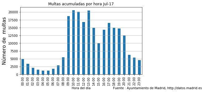
Veamos la distribución de multas por hora : (recordamos de nuevo que en esta gráfica se representa el acumulado en esa hora de todos los dias del mes)
multas_hist=multas['hora_entera'].value_counts().sort_index(axis=0)

fig = plt.figure(1, (7,4))
ax = fig.add_subplot(1,1,1)
ax=multas_hist.plot.bar()
ax.locator_params(axis='y',nbins=10)
ax.set_xlabel('Hora del día')
ax.set_ylabel('Número de multas',size=16)
ax.grid(axis='y')
ax.set_title('Multas acumuladas por hora Jul-17')
fig.suptitle(fuente,size=10,x=1,y=-0.01)
fig.savefig('multas_hora_Jul17',bbox_inches = 'tight')
Con porcentajes en vez de números absolutos :
multas_hist_porcentaje=multas['hora_entera'].value_counts().sort_index(axis=0)/len(multas)*100
fig = plt.figure(1, (7,4))
ax = fig.add_subplot(1,1,1)
ax=multas_hist_porcentaje.plot.bar()
ax.locator_params(axis='y',nbins=10)
ax.set_xlabel('Hora del día')
ax.set_ylabel('% multas',size=16)
ax.grid(axis='y')
ax.set_title('Porcentajes de multas en cada hora Jul-17')
fmt = '%3.1f%%'
yticks = mtick.FormatStrFormatter(fmt)
ax.yaxis.set_major_formatter(yticks)
fig.suptitle(fuente,size=10,x=1,y=-0.01)
fig.savefig('multas_hora_porcentaje_Jul17',bbox_inches = 'tight')

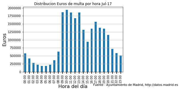
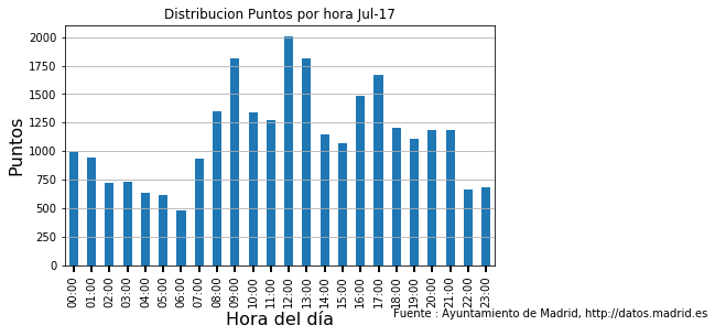
Seguimos con la distribución de euros y puntos perdidos por hora :
multas_euros=multas.sort_values('HORA').groupby("hora_entera",sort=False).IMP_BOL
fig1 = plt.figure()
ax1 = fig1.add_subplot(1,1,1)
ax1 = multas_euros.sum().plot.bar()
ax1.locator_params(axis='y',nbins=10)
ax1.set_xlabel('Hora del día',size=16)
ax1.set_ylabel('Euros',size=16)
ax1.tick_params(axis='x',direction='out', length=6, width=2, colors='black')
#ax1.set_xticklabels(multas_euros['hora_entera'])
ax1.grid(axis='y')
ax1.set_title('Distribucion Euros de multa por hora Jul-17')
fig1.suptitle(fuente,size=10,x=1,y=-0.01)
fig.savefig('euros_hora',bbox_inches = 'tight')
multas_puntos=multas.sort_values('HORA').groupby("hora_entera",sort=False).PUNTOS
fig1 = plt.figure(1,(7,4))
ax1 = fig1.add_subplot(1,1,1)
ax1 = multas_puntos.sum().plot.bar()
ax1.locator_params(axis='y',nbins=10)
ax1.set_xlabel('Hora del día',size=16)
ax1.set_ylabel('Puntos',size=16)
ax1.tick_params(axis='x',direction='out', length=6, width=2, colors='black')
#ax1.set_xticklabels(multas_euros['hora_entera'])
ax1.grid(axis='y')
ax1.set_title('Distribucion Puntos por hora Jul-17')
fig1.suptitle(fuente,size=10,x=1,y=-0.01)
fig1.savefig('puntos_hora_Jul17',bbox_inches = 'tight')
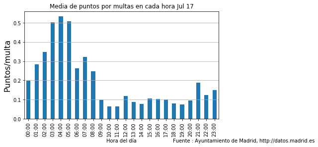
He calculado un par de ratios de interés, euros por multa y puntos por multa a lo largo del día, viendo que la media por la noche es significativamente superior a la media del día. Aquí vemos exclusivamente que las multas de la noche traen más euros y quitan as puntos que las multas de día, cosa que parece razonable, en ambos casos vemos que la hora caliente es de 04:00 a 05:00 de la madrugada, con más de 160€ y casi 0.6 puntos por multa.
ratio_euros_multas=multas_euros.sum()/multas_hist
fig = plt.figure(1, (7,4))
ax = fig.add_subplot(1,1,1)
ax=ratio_euros_multas.plot.bar()
ax.locator_params(axis='y',nbins=10)
ax.set_xlabel('Hora del día')
ax.set_ylabel('€/multa',size=16)
ax.grid(axis='y')
ax.set_title('Media de € por multa Jul-17')
fig.suptitle(fuente,size=10,x=1,y=-0.01)
fig.savefig('media_euros_multa_Jul17',bbox_inches = 'tight')

ratio_puntos_multas=multas_puntos.sum()/multas_hist
fig = plt.figure(1, (7,4))
ax = fig.add_subplot(1,1,1)
ax=ratio_puntos_multas.plot.bar()
ax.locator_params(axis='y',nbins=10)
ax.set_xlabel('Hora del día')
ax.set_ylabel('Puntos/multa',size=16)
ax.grid(axis='y')
ax.set_title('Media de puntos por multas en cada hora Jul 17')
fig.suptitle(fuente,size=10,x=1,y=-0.01)
fig.savefig('media_puntos_multa_Jul17',bbox_inches = 'tight')
Toca ahora analizar las multas según su tipo, siguiendo con la terminología del fichero : con el HECHO_BOL, el hecho descrito en el boletín de multa. Empezamos por las multas más frecuentes según tipo, podemos ver que más de 55000 multas vienen de saltarse las restricciones de trafico en zonas con circulación limitado, como ejemplo el centro de MAdrid. Analizaremos en profundidad este hecho en otro post. Continuaremos con un par de tablas con los puntos y euros de los hechos de multas que más puntos retiran (slatarse un semaforo en rojo) y euros recaudan (circular por zonas limitadas), y esas mismas tablas pasadas a gráficos.
multas_hecho=multas.HECHO_BOL.value_counts()
fig = plt.figure(1, (7,4))
ax = fig.add_subplot(1,1,1)
ax=multas_hecho.head(10).plot.barh()
ax.locator_params(axis='y',nbins=10)
ax.locator_params(axis='x',nbins=20)
ax.set_xlabel('Número de multas',size=20)
ax.grid(axis='x')
ax.invert_yaxis()
ax.set_yticklabels(['{:>80}'.format(x.strip()[:80]) for x in multas_hecho.index],size=10)
ax.set_title('Hechos denunciados más frecuentes Jul-17')
fig.suptitle(fuente,size=10,x=1,y=-0.01)
fig.savefig('hechos_fecuentes_Jul17',bbox_inches = 'tight')


multas_hecho_importe=multas.groupby('HECHO_BOL')
multas_hecho_importe['IMP_BOL','PUNTOS'].sum().sort_values('PUNTOS',ascending=False).reset_index().head()
| HECHO_BOL | IMP_BOL | PUNTOS | |
|---|---|---|---|
| 0 | SOBREPASAR LA VELOCIDADMÁXIMA EN VÍAS LIMITADA… | 2,014,600.0 | 8786 |
| 1 | REBASAR UN SEMÁFORO EN FASE ROJA. … | 426,800.0 | 8332 |
| 2 | UTILIZAR MANUALMENTE PANTALLAS, NAVEGADORES, D… | 157,600.0 | 2331 |
| 3 | CONDUCIR CON UNA TASA DE ALCOHOLEMIA NO PERMIT… | 289,000.0 | 1692 |
| 4 | SOBREPASAR LA VELOCIDADMÁXIMA EN VÍAS LIMITADA… | 4,243,700.0 | 1532 |
multas_hecho_importe['IMP_BOL','PUNTOS'].sum().sort_values('IMP_BOL',ascending=False).reset_index().head()
| HECHO_BOL | IMP_BOL | PUNTOS | |
|---|---|---|---|
| 0 | NO RESPETAR LAS SEŃALES EN UNA VÍA DE CIRCULAC… | 5,168,520.0 | 0 |
| 1 | ESTACIONAR, SIN LA CORRESPONDIENTE AUTORIZACIÓ… | 4,272,390.0 | 0 |
| 2 | SOBREPASAR LA VELOCIDADMÁXIMA EN VÍAS LIMITADA… | 4,243,700.0 | 1532 |
| 3 | SOBREPASAR LA VELOCIDADMÁXIMA EN VÍAS LIMITADA… | 2,014,600.0 | 8786 |
| 4 | ESTACIONAR EN LUGAR PROHIBIDO DEBIDAMENTE SEŃA… | 1,230,210.0 | 0 |
pd_aux=multas_hecho_importe['PUNTOS'].aggregate('sum').sort_values(ascending=False).head(7)
N=5
width=.5
ind = np.arange(len(pd_aux))
fig, ax = plt.subplots()
rects = ax.barh(ind, pd_aux.values, width, align='center',color='b', label='Puntos')
ax.set_title('Simple plot')
ax.set_ylabel('Concepto de multa',size=20)
ax.set_xlabel('Acumulado euros de multas',size=16)
ax.set_yticks(ind)
ax.set_yticklabels(['{:>80}'.format(x.strip()[:80]) for x in pd_aux.index],
size=12,rotation=0,color='b')
ax.invert_yaxis()

ax.grid(axis='x')
ax.set_title('Puntos por tipo multa Jul-17')
ax.legend()
fig.suptitle(fuente,size=10,x=1,y=-0.01)

for rect in rects:
width = rect.get_width()
plt.text(width,rect.get_y()+rect.get_height()/2 ,'%1.1f%%' % (100*width/puntos_totales), size=16, ha='left', va='center')

plt.show()
fig.savefig('puntos_hecho_multa_Jul17',bbox_inches = 'tight')

Redondeando podemos ver que el 32% de los puntos retirados se pierden por correr en zonas de tráfico limitado a 50km/h..
pd_aux=multas_hecho_importe['IMP_BOL'].aggregate('sum').sort_values(ascending=False).head(10)
N=5
width=.5
ind = np.arange(len(pd_aux))
fig = plt.figure(1, (10,7))
ax = fig.add_subplot(1,1,1)

rects = ax.barh(ind, pd_aux.values, width, align='center',color='b', label='Euros')
ax.set_title('Simple plot')
ax.set_ylabel('Concepto de multa',size=20)
ax.set_xlabel('Acumulado euros de multas',size=16)
ax.set_yticks(ind)
ax.set_yticklabels(['{:>120}'.format(x.strip()[:120]) for x in pd_aux.index],
size=16,rotation=0,color='b')
ax.invert_yaxis()

ax.grid(axis='x')
ax.set_title('Euros por tipo multa')
ax.legend()
fig.suptitle(fuente,size=16,x=1,y=-0.01)

for rect in rects:
width = rect.get_width()
plt.text(width,rect.get_y()+rect.get_height()/2 ,'%1.1f%%' % (100*width/euros_totales), size=20, ha='left', va='center')

plt.show()
fig.savefig('euros_hecho_multa_Jul17',bbox_inches = 'tight')

..y el 22% de los euros recaudados vienen de multas por circular en zonas restriguidas.
Y finalmente analizaremos las multas de velocidad.
Empezamos haciendo un filtro :
multas_filtrada_velocidad=multas[multas.velocidad_circulacion!=0]
Calculando el tamaño del nuevo pandas vemos que hay 53.243 multas de velocidad.
multas_de_velocidad=len(multas_filtrada_velocidad)
multas_de_velocidad
53243
Saquemos unos cálculos interesantes
multas_filtrada_velocidad.groupby('velocidad_limite')['velocidad_circulacion'].describe()
| count | mean | std | min | 25% | 50% | 75% | max | |
|---|---|---|---|---|---|---|---|---|
| velocidad_limite | ||||||||
| 40 | 206.0 | 63.8 | 6.9 | 54.0 | 59.0 | 62.0 | 68.0 | 88.0 |
| 50 | 12,073.0 | 67.9 | 6.9 | 53.0 | 63.0 | 66.0 | 71.0 | 100.0 |
| 60 | 364.0 | 84.3 | 8.8 | 70.0 | 77.0 | 83.0 | 90.0 | 114.0 |
| 70 | 34,826.0 | 79.6 | 6.5 | 74.0 | 75.0 | 77.0 | 82.0 | 136.0 |
| 80 | 20.0 | 98.8 | 6.2 | 93.0 | 94.8 | 97.5 | 101.0 | 117.0 |
| 90 | 5,754.0 | 100.4 | 6.1 | 95.0 | 96.0 | 99.0 | 102.0 | 152.0 |
Aquí podemos ver algunas características de las multas de velocidad ordenadas por la velocidad límite. Con algunas curiosidades a primera vista : la mayor parte de las multas se consiguen en zonas con 70 km/h de velocidad límite..Se ha multado a 53km/h en zonas de 50km/hr, sin embargo no se ha multado hasta los 93km/h en zona de 80km/h..aunque cierto es que el número de multas a 80km/h es despreciable : 20 de las 44.659…
Veamoslo en gráficos : número de multas
multas_filtrada_velocidad['velocidad_limite'].sort_values().unique()
array([40, 50, 60, 70, 80, 90])
multas_filtrada_velocidad.groupby('velocidad_limite')['velocidad_circulacion'].count()
velocidad_limite
40 206
50 12073
60 364
70 34826
80 20
90 5754
Name: velocidad_circulacion, dtype: int64
fig = plt.figure(1, (12,7))
width=.8
ind = np.arange(len(multas_filtrada_velocidad.groupby('velocidad_limite')['velocidad_circulacion'].aggregate('count')))

ax = fig.add_subplot(111)

rects = ax.bar(ind, multas_filtrada_velocidad.groupby('velocidad_limite')['velocidad_circulacion'].aggregate('count'),
width, align='center',color='b', label='nº multas')

ax.set_xticks(ind)
ax.set_xticklabels([x for x in multas_filtrada_velocidad['velocidad_limite'].sort_values().unique()],
size=12,rotation=0,color='b')
ax.set_xlabel('Velocidad límite en km/h')
ax.set_ylabel('Número de multas',size=16)
ax.grid(axis='y')
ax.set_title('Número de multas de velocidad por velocidad límite Jul-17')
ax.legend()
fig.suptitle(fuente,size=10,x=1,y=-0.01)

for rect in rects:
height = rect.get_height()
plt.text(rect.get_x()+rect.get_width()/2,height ,'%1.1f%%' % (100*height/multas_de_velocidad), size=10, ha='center', va='bottom')

plt.show()
fig.savefig('multas_velocidad_limite_Jul17',bbox_inches = 'tight')

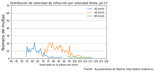
..y un par de gráficas adicionales con la distribución de velocidad que llevaban los multados frente ordenados por la velocidad límite :
fig = plt.figure(1, (7,4))
ax = fig.add_subplot(1,1,1)
ax.plot(
multas_filtrada_velocidad[multas_filtrada_velocidad['velocidad_limite']==50]['velocidad_circulacion'].sort_values().unique(),
multas_filtrada_velocidad[multas_filtrada_velocidad['velocidad_limite']==50].groupby('velocidad_circulacion')['velocidad_circulacion'].count(),
label='50 km/h',
)

ax.plot(
multas_filtrada_velocidad[multas_filtrada_velocidad['velocidad_limite']==70]['velocidad_circulacion'].sort_values().unique(),
multas_filtrada_velocidad[multas_filtrada_velocidad['velocidad_limite']==70].groupby('velocidad_circulacion')['velocidad_circulacion'].count(),
label='70 km/h',
)
ax.plot(
multas_filtrada_velocidad[multas_filtrada_velocidad['velocidad_limite']==90]['velocidad_circulacion'].sort_values().unique(),
multas_filtrada_velocidad[multas_filtrada_velocidad['velocidad_limite']==90].groupby('velocidad_circulacion')['velocidad_circulacion'].count(),
label='90 km/h',
)

ax.locator_params(axis='x',nbins=20)
ax.set_xlabel('Velocidad en la infracción km/h')
ax.set_xlim([50,160])
ax.set_ylim([0,7000])
ax.set_ylabel('Número de multas',size=16)
ax.grid(axis='y')
ax.set_title('Distribución de velocidad de infracción por velocidad límite Jul-17')
ax.legend()

fig.suptitle(fuente,size=10,x=1,y=-0.01)
fig.savefig('distribucion_velocidad_507090_Jul17',bbox_inches = 'tight')
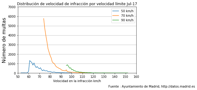
fig = plt.figure(1, (7,4))
ax = fig.add_subplot(1,1,1)
ax.plot(
multas_filtrada_velocidad[multas_filtrada_velocidad['velocidad_limite']==40]['velocidad_circulacion'].sort_values().unique(),
multas_filtrada_velocidad[multas_filtrada_velocidad['velocidad_limite']==40].groupby('velocidad_circulacion')['velocidad_circulacion'].count(),
label='40 km/h',
)

ax.plot(
multas_filtrada_velocidad[multas_filtrada_velocidad['velocidad_limite']==60]['velocidad_circulacion'].sort_values().unique(),
multas_filtrada_velocidad[multas_filtrada_velocidad['velocidad_limite']==60].groupby('velocidad_circulacion')['velocidad_circulacion'].count(),
label='60 km/h',
)
ax.plot(
multas_filtrada_velocidad[multas_filtrada_velocidad['velocidad_limite']==80]['velocidad_circulacion'].sort_values().unique(),
multas_filtrada_velocidad[multas_filtrada_velocidad['velocidad_limite']==80].groupby('velocidad_circulacion')['velocidad_circulacion'].count(),
label='80 km/h',
)

ax.locator_params(axis='x',nbins=20)
ax.set_xlabel('Velocidad en la infracción km/h')
ax.set_xlim([40,130])
ax.set_ylim([0,70])
ax.set_ylabel('Número de multas',size=16)
ax.grid(axis='y')
ax.set_title('Distribución de velocidad de infracción por velocidad límite, Jul-17')
ax.legend()

fig.suptitle(fuente,size=10,x=1,y=-0.01)
fig.savefig('dsitribibucion_velocidad_406080_Jul17',bbox_inches = 'tight')
Con el afan de ver las multas «extremas», no en absoluto si no con el ratio velocidad_circulacion/velocidad/limite, introducimos una nueva columna…
multas_filtrada_velocidad['ratio']=multas_filtrada_velocidad['velocidad_circulacion']/multas_filtrada_velocidad['velocidad_limite']
/Users/waly/anaconda/envs/OpenData/lib/python3.6/site-packages/ipykernel_launcher.py:1: SettingWithCopyWarning:
A value is trying to be set on a copy of a slice from a DataFrame.
Try using .loc[row_indexer,col_indexer] = value instead
See the caveats in the documentation: http://pandas.pydata.org/pandas-docs/stable/indexing.html#indexing-view-versus-copy
«»»Entry point for launching an IPython kernel.
y vemos los casos extremos (head y tail)..
En la parte alta : multa catalogada como GRAVE a 88 km/hr en zona de 40km/h en la Avenida Séneca con velocida máxima 40km/h, a las 17:05…otros 500€ del ala!
..y en la parte baja : multa a 95km/h en el km de la M-30, km 27, en zona de 90km/h a las 18:23..100€ por esos 5 km/h
multas_filtrada_velocidad.sort_values('ratio',ascending=False).head(2)
| CALIFICACION | LUGAR | MES | ANIO | HORA | IMP_BOL | DESCUENTO | PUNTOS | DENUNCIANTE | HECHO_BOL | VEL_LIMITE | VEL_CIRCULA | COORDENADA_X | COORDENADA_Y | hora_entera | velocidad_limite | velocidad_circulacion | ratio | |
|---|---|---|---|---|---|---|---|---|---|---|---|---|---|---|---|---|---|---|
| 231825 | GRAVE | S/N AV SENECA | 7 | 2017 | 1900-01-01 17:05:00 | 500.0 | SI | 6 | POLICIA MUNICIPAL | SOBREPASAR LA VELOCIDADMÁXIMA EN VÍAS LIMITADA… | 40 | 88 | 17:00 | 40 | 88 | 2.2 | ||
| 115695 | GRAVE | F081 PO ERMITA DEL SANTO | 7 | 2017 | 1900-01-01 12:25:00 | 500.0 | SI | 6 | POLICIA MUNICIPAL | SOBREPASAR LA VELOCIDADMÁXIMA EN VÍAS LIMITADA… | 40 | 88 | 12:00 | 40 | 88 | 2.2 |
multas_filtrada_velocidad.sort_values('ratio',ascending=False).tail(2)
| CALIFICACION | LUGAR | MES | ANIO | HORA | IMP_BOL | DESCUENTO | PUNTOS | DENUNCIANTE | HECHO_BOL | VEL_LIMITE | VEL_CIRCULA | COORDENADA_X | COORDENADA_Y | hora_entera | velocidad_limite | velocidad_circulacion | ratio | |
|---|---|---|---|---|---|---|---|---|---|---|---|---|---|---|---|---|---|---|
| 231079 | GRAVE | M-30 CALZADA 2 KM 27.000 | 7 | 2017 | 1900-01-01 18:23:00 | 100.0 | SI | 0 | POLICIA MUNICIPAL | SOBREPASAR LA VELOCIDADMÁXIMA EN VÍAS LIMITADA… | 90 | 95 | 18:00 | 90 | 95 | 1.1 | ||
| 168620 | GRAVE | M-30 C-2 KM 7,800 CR-CRA | 7 | 2017 | 1900-01-01 02:28:00 | 100.0 | SI | 0 | POLICIA MUNICIPAL | SOBREPASAR LA VELOCIDADMÁXIMA EN VÍAS LIMITADA… | 90 | 95 | 02:00 | 90 | 95 | 1.1 |
<br />
